Introduction
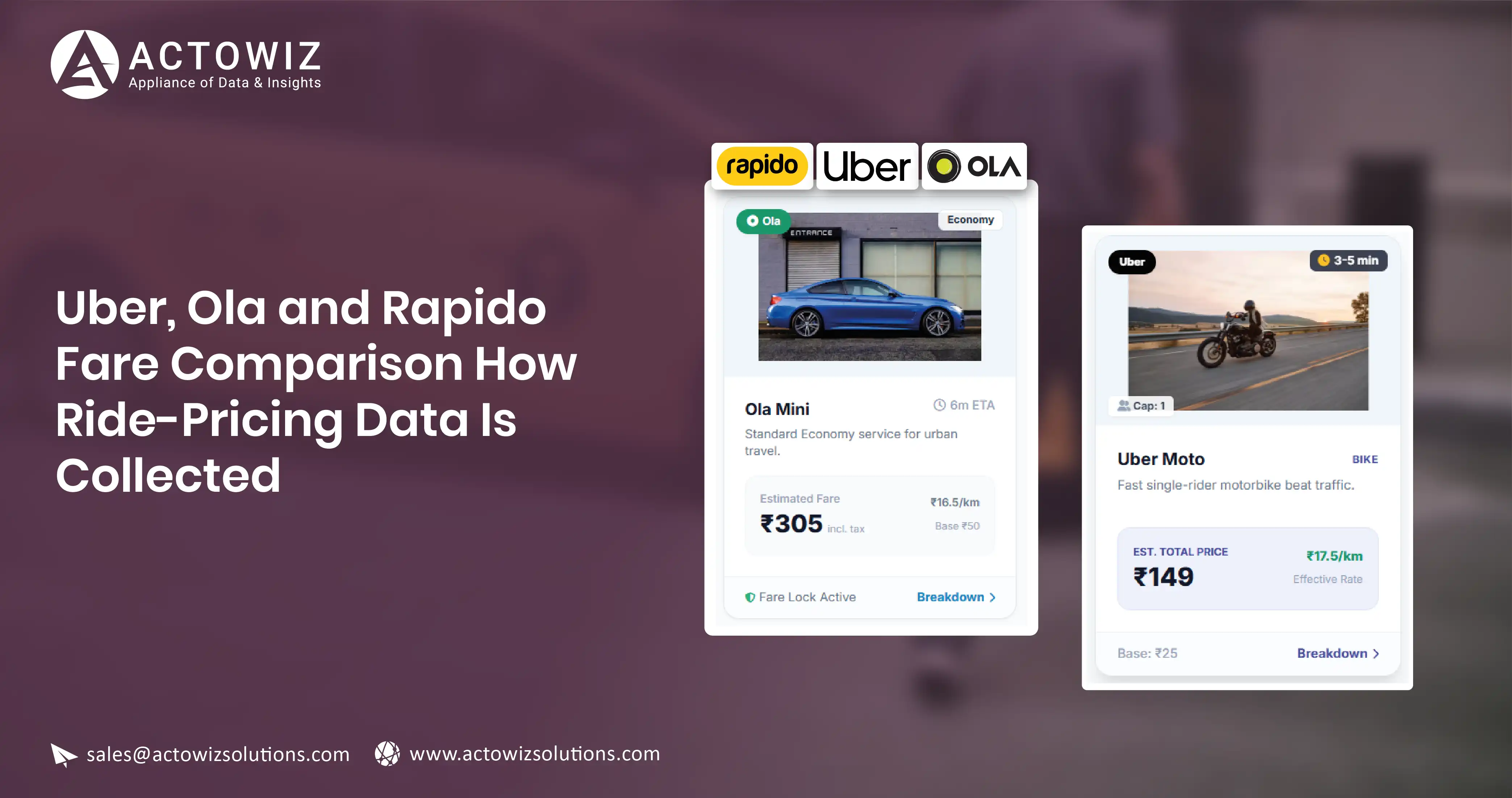
There is no price list for a ride. A hotel publishes a rate. A retailer publishes a product page. A ride-hailing app publishes nothing until you name an origin, a destination and a moment — and then it gives you one quote, valid for that combination only.
That single fact changes the entire collection design. You are not crawling a catalogue and you never will be. You are constructing a measurement matrix and sampling it repeatedly.
This post covers how to build that matrix, how to handle surge, how to map vehicle categories across three apps that name their tiers differently, and why the average fare is almost always the wrong output. Our mobile app data collection and travel and mobility data services are built on this matrix design rather than assuming a crawlable catalogue.
Why ride pricing has no catalogue
Every fare quote is a function of at least these inputs, most of which are outside your control:
- Origin coordinate and destination coordinate
- Time of request
- Live supply of drivers near the origin
- Live demand in the same area
- Vehicle category requested
- Route the app's engine selects, which affects distance and duration estimates
- Any active promotion or dynamic multiplier
Change the minute and the answer changes. Change the pickup point by 300 metres and the answer can change. There is no stable object to crawl, so there is nothing to enumerate.
The consequence: your dataset's quality is determined almost entirely by sampling design. A badly designed matrix collected millions of times is still a badly designed matrix.
Designing the route × time-slot matrix
The unit of analysis is a cell: one origin-destination pair, one vehicle category, one time slot, one app. You sample cells repeatedly and study the distribution inside each.
Choosing routes
Pick routes that represent distinct pricing regimes, not routes that are merely busy.
| Route archetype |
What it measures |
Notes |
| Airport to CBD |
High-value, supply-constrained runs |
Often has its own pricing rules and pickup zones |
| CBD pair, short |
Dense-supply short-haul behaviour |
Most sensitive to surge |
| Residential to commercial |
Commute-direction asymmetry |
Run in both directions as separate cells |
| Suburb to suburb, long |
Long-haul per-km behaviour |
Where category pricing diverges most |
| Transit hub to residential |
Last-mile behaviour |
Where two-wheeler and auto tiers matter most |
| Low-density outer route |
Supply scarcity and unavailability |
Produces the no-quote cases you need |
A workable starting scope is 12 to 20 routes per city. Fewer than about 10 and you cannot separate route effects from time effects. More than about 25 and the time-slot dimension usually gets sacrificed, which is the worse trade.
Two design rules that are easy to get wrong:
Fix the exact coordinates, not the place name. Store a pinned latitude and longitude for each endpoint and reuse it forever. A named landmark can resolve to different pickup points across apps and across releases, which silently changes the route.
Treat each direction as its own route. Commute-hour pricing is asymmetric. Averaging the two directions destroys the effect you most want to see.
Coordinate resolution, pinning and geography masters are covered in our geo and location data collection service.
Choosing time slots
Time slots are where the signal lives. A minimum viable set for an Indian metro:
| Slot |
Window |
Why |
| Early morning |
05:30–07:00 |
Airport runs, low supply |
| Morning peak |
08:30–10:30 |
Commute demand |
| Midday off-peak |
12:30–15:00 |
Baseline reference |
| Evening peak |
17:30–20:30 |
Highest and most variable |
| Late evening |
21:30–23:00 |
Thinning supply |
| Late night |
00:30–03:00 |
Night pricing rules, sparse supply |
Sample each slot on multiple days, and keep weekday and weekend as separate strata. A Tuesday evening peak and a Saturday evening peak are different phenomena.
Repetition inside a slot is what makes the data usable. One quote per slot per day tells you very little. Three to five quotes spaced within the slot, across at least two weeks, gives you a distribution you can describe.
So the matrix size is roughly: routes × directions × categories × slots × repetitions × days × apps. Keep it deliberately small in the route dimension so the repetition dimension can be generous.
Surge is the dominant variance
On most routes in most cities, the spread within a single cell is wider than the difference between apps. Surge, or whatever each platform calls its dynamic component, is the main driver.
Three ways surge is exposed, in descending order of usefulness:
- An explicit multiplier or surcharge line shown in the quote. Capture it verbatim.
- A qualitative indicator — a notice that prices are higher than usual. Capture as a boolean plus the raw text.
- Nothing at all, with the surge baked into the fare. Then you infer it from the cell's own baseline.
For case three, build a per-cell baseline from the off-peak slot for that route, direction and category, using a low percentile of observed fares over a rolling window. Express each observation as a ratio to that baseline. That ratio is your surge proxy.
Two cautions. The baseline must be per-cell, not per-city, because per-km economics differ by route. And the proxy is a derived field — store it separately from observed fields, and never present it as something the app disclosed.
Mapping vehicle categories across apps
Three apps, three naming schemes, overlapping but not identical products. This is a normalisation problem, and getting it wrong invalidates every cross-app comparison.
Build a controlled vocabulary based on the physical product, not the brand name:
| Normalised category |
Defining attributes |
Notes |
| two_wheeler |
Motorcycle, single pillion rider |
Availability varies by city and regulation |
| auto_three_wheeler |
Three-wheeler, up to 3 passengers |
Often metered differently from cars |
| hatchback_economy |
Compact car, up to 4 passengers |
The volume tier in most cities |
| sedan_standard |
Sedan, up to 4 passengers |
|
| suv_large |
6 to 7 passengers |
|
| premium |
Higher-spec vehicle, same capacity as sedan |
Availability is patchy |
| rental_or_outstation |
Package products, not point-to-point |
Exclude from point-to-point comparisons |
Then hold a mapping table from each app's displayed tier name to a normalised category, with a version and an effective date. Apps rename and reshuffle tiers. A versioned mapping lets you reprocess history correctly instead of retro-fitting a guess.
Two rules keep the mapping honest. Never map a product whose passenger capacity or vehicle class differs — an unmapped row is better than a wrong one. And exclude package products entirely from point-to-point analysis; they price on time and distance allowances, not on the trip.
The field schema
| Field |
Type |
Notes |
| observation_id |
string |
Unique per quote |
| sweep_id |
string |
Groups quotes taken across apps in one window |
| app_name |
string |
Platform observed |
| city |
string |
Normalised city name |
| route_id |
string |
Stable ID for the pinned OD pair and direction |
| origin_lat / origin_lng |
decimal |
Pinned, never re-geocoded |
| dest_lat / dest_lng |
decimal |
Pinned |
| route_archetype |
enum |
From the archetype table |
| distance_km_quoted |
decimal, nullable |
As the app estimates it |
| duration_min_quoted |
integer, nullable |
As the app estimates it |
| vehicle_tier_raw |
string |
Displayed tier name, verbatim |
| vehicle_category_normalised |
enum |
From the controlled vocabulary |
| mapping_version |
string |
Version of the tier mapping applied |
| quoted_fare |
decimal, nullable |
Total quoted to the rider |
| fare_is_range |
boolean |
Some quotes are a band, not a point |
| fare_low / fare_high |
decimal, nullable |
Populated when a range is shown |
| currency |
string |
ISO code |
| surge_indicator_present |
boolean |
Explicit dynamic-pricing notice shown |
| surge_multiplier_stated |
decimal, nullable |
Only when the app states it |
| surge_notice_text |
string, nullable |
Raw text, unparsed |
| eta_pickup_min |
integer, nullable |
Estimated wait for pickup |
| availability_status |
enum |
quoted / no_vehicles / not_serviceable / error |
| promo_applied_flag |
boolean |
Any visible discount applied |
| time_slot |
enum |
From the slot table |
| day_type |
enum |
weekday / weekend / public_holiday |
| collected_at |
timestamp |
UTC, to the second |
Two notes on the schema.
availability_status is a first-class field, not an error state. A route that cannot be served at 02:00 is a finding. Dropping those rows makes late-night pricing look better than it is.
sweep_id is what makes cross-app comparison legitimate. Quotes for the same route pulled at 18:05 and 18:40 are not comparable. Group them into a sweep and discard sweeps that did not complete within a tight window — a few minutes at most.
Why the average fare is nearly useless
Take one cell: airport to CBD, sedan, evening peak. Collect it for three weeks. The fares will not cluster around a mean. They will be bimodal or heavily right-tailed, because some observations landed in surge and some did not.
The mean sits in a gap where few actual fares occur. Report it and you describe a fare nobody paid.
The distribution is the answer. Useful outputs per cell:
- Median fare
- 10th and 90th percentile, giving the realistic range
- Interquartile range as a volatility measure
- Share of observations above 1.5× the cell baseline, as a surge frequency
- Share of observations with availability_status other than quoted
- Median eta_pickup_min, which often matters more than price
For cross-app work, compare the same percentile across apps within the same sweeps: median and 90th-percentile quoted fare by app, normalised category and time slot, selected city. Comparing App A's mean to App B's mean across different sweeps compares two different sets of moments.
Failure modes worth naming: re-geocoded endpoints silently changing the route; unversioned tier mappings corrupting history; promo-discounted quotes entering the baseline; sweeps stretched over an hour; and dropped no-quote rows inflating apparent availability.
ETA belongs in the analysis, not the footnotes
Price is the field everyone asks for. Wait time is often the field that decides the trip.
A fare that is 15 percent lower with a 14-minute pickup wait is not a better offer than a slightly higher fare arriving in 3 minutes, and no rider treats it as one. If your dataset carries eta_pickup_min but your analysis ignores it, you are describing a market nobody is actually choosing in.
Two useful framings:
Cost per minute of total journey. Combine the quoted fare with pickup ETA plus quoted duration. This penalises cheap-but-distant supply and makes cross-app comparisons closer to the rider's real trade-off.
Effective availability. A route where quotes exist but pickup ETAs routinely exceed some threshold is functionally underserved, even though availability_status reads quoted on every row. Report the share of observations above an ETA threshold alongside the no-quote share; together they describe service coverage far better than either alone.
ETA is also the field most sensitive to the pinned coordinate. Moving a pickup point across a road divider or outside a restricted airport zone changes wait times substantially. This is the strongest practical argument for pinning coordinates once and never re-geocoding them.
Who uses this data
- Mobility analysts and transport researchers need per-cell distributions to study affordability and supply gaps across a city.
- Corporate travel and expense teams need percentile fares by route and slot to set realistic reimbursement bands rather than flat caps.
- City transport and policy research needs availability and ETA data as much as fares, since unserved areas are the policy question.
- Operators benchmarking competitors need same-sweep comparisons on a fixed route panel, with categories normalised, so a difference is attributable to pricing rather than timing.
Actowiz Solutions builds ride-pricing collection to a defined route and time-slot matrix, with pinned coordinates, versioned vehicle-tier mapping, sweep grouping for cross-app comparability, and availability captured as a field rather than discarded. Delivery is as a scheduled feed, an API, or distribution-level aggregates. The scheduling and live-collection side is covered in our live collection infrastructure and continuous price monitoring services, with city-level collection described in data collection across Indian cities.
We collect from public-facing quote surfaces and record the exact conditions of each quote, so what you report is a measured distribution rather than a single number.
You can also reach us for all your mobile app scraping, data collection, web scraping, and instant data scraper service requirements!
FAQ
1. Why is a route by time-slot matrix used instead of crawling ride fares?
Because ride fares are quotes generated per request, not published listings. There is no catalogue to enumerate. Data quality therefore depends on which origin-destination pairs, vehicle categories and time windows you choose to sample, and how often you repeat each cell.
2. How are vehicle categories compared across apps with different tier names?
Through a versioned mapping table that translates each app's displayed tier into a normalised category defined by vehicle class and passenger capacity. Products that do not match on those attributes are left unmapped rather than forced, and package or outstation products are excluded from point-to-point comparisons.
3. Why is the average fare a poor summary of ride-pricing data?
Because fares within a single route and time slot are usually right-tailed or bimodal, depending on whether dynamic pricing was active. The mean falls in a range where few real fares occur. Median, 10th and 90th percentiles, and the share of surge observations describe the data far better.
 Actowiz Solutions

 By industry
 Pricing & Promotions
 Brand & Intelligence
 Digital Shelf & Search
 Assortment
 For Retailers
 E-Commerce Dashboard
 Flipkart Insights (Live)
 Grocery Intelligence
.svg) Grocery Price (U.S.)
.svg) Quick Commerce (India)
 Food & Restaurant
 Fashion Intelligence
 Automotive
 Travel & Hospitality
 Real Estate
 Food Delivery Intelligence
 OTT & Streaming
 Fuel & EV Charging Price Tracker
 By Use Case
 Pricing Intelligence
 Digital Shelf Analytics
 MAP Monitoring
 Cross-Border Price Parity
 Share of Search
 Review Sentiment
 Kitchen Market Gaps
 Dynamic Pricing / AI Repricing
 Promotions & Deals Alerts
 B2B / POI & Lead Data
 AI Search Visibility Dashboard
 Baby Products on Quick Commerce
 Hotel & Flight Rate Parity
 By Region
 Flipkart Real-Time Insights
 Quick Commerce — Zepto · Blinkit
 Pincode Price Tracker
 GCC Q-Commerce — Talabat · Noon
 UK Grocery — Tesco, Sainsbury's, Asda
 AU Grocery — Coles & Woolworths
 Marketplace Scrapers
 Developer APIs
 Universal APIs
 Delivery & SDKs
 Knowledge Center
 Guides & Playbooks
 Downloads & Tools
 Trust & Company


 4.8/5 Average Rating
 50+ Video Testimonials
 92% Client Retention
 50+ Countries Served